In this Excel tutorial wage system employees are given incentive for increased
productivity. In this system different tiers slabs or scales of output
are defined and progressive slab has increased wage rate.
Calculating wages in this system is not simple as it was in earlier cases. Because in this situation first we have to identify the number of units employee has identified. Then we have to look up for the slab in which that output falls and take the rate of that slab and apply it to calculate wage.
Excel have functions or formula that do exactly the same and are called LOOKUP functions. We have different variants of these but the one I will be using is VLOOKUP.
In this situation we have slabs as follows:
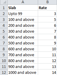
Step 2: Right click on any cell in Rate column. From the menu click “insert”The information of slabs is not in the form that we can use in the formula. We need only numbers. For this purpose we will add another column between Slab and Rate column named Class. To add column in between follow these steps:
Step 3: An insert dialogue box will appear. From the dialogue box select “Entire column” and click OK.
New column will be added between Slabs and column. Name the column “Class” and type 0, 100, 200…., 1000 in the column as shown below:

Observe the slabs. In this data 1-99 is one slab 100-199 is another slab. But how do excel knows this? Well the formula we are about to use understands this automatically as it is programmed like this. If employee has produced 95 units. It will go to 100 and see its on the next level so it will revert back to previous rate. So automatically it will stay within 1-99 range for 3 dollars rate.
Step 4: With the data ready to be used, we have employee information in with their names and units produced put the following formula in cell G5:
=F5*VLOOKUP(F5,B5:C15,2)
Press enter and wage of first employee is done. Drag the fill handler down or double click to process wages for the rest of employees as well.
In this formula B19 contains the value of units produced which we know before hand multiplied with the appropriate rate for which we found using VLOOKUP function. And this solves our case.
Steps to enter above formula:
Step 1: Select cell and press = button. This will put excel in edit mode.
Step 2: Write B19 or select the value of units produced by first employee.
Step 3: Press and hold Shift button and hit 8 on the keyboard this will put asterisk * in the formula that works as multiply in mathematics.
Step 4: Type vlookup. Notice when you were typing the helper tag appears just under the field where you type a smart tip appears. You can make the selection of right function using directional arrows. Once VLOOKUP highlighted press TAB key on the keyboard.
Step 5: Select the same cell again i.e. units produced as you will use units produced to look up for the slab and hit comma button. Mostly found just at the left to enter key.
Step 6: Select the data in Class and Rate column with mouse. Lock the range i.e. make it absolute by cursor in or with the range and press F4 function key one time. This will put $ sign with the column and row references. Once done hit comma button on the keyboard.
Step 7: The target information is in the second column of selected range so press 2 key on the keyboard.
Step 8: Press and hold shift key and press 0 (zero) key to put closing parenthesis and hit Enter key.
To best practice all the above steps use the following worksheet. Few steps have already been done for you:
Differential piece work wage payment – Case 2
Make sure the worksheet named: DPW – S2
In previous example our scale was set like 0-99, 100-199 and so on. Meaning everyone hundredth value was in the next slab. But what if we want the data to be like; 0-100, 101-200 and so on. In other words instead of 100 and above, 200 and above, 300 and above we want Upto 100, Upto 200, Upto 300 etc. This changes the scenario a little bit as previously 100, 200, 300 were in next slabs but in this case they are in the same slab.
To incorporate this we only have to change our range a little bit and rest of the steps are same as above. Instead of having classes as 0, 100, 200 and so on. Now the classes will be 0, 101, 201, 301 and so on. This way for 0-100 applicable rate will be 3, 101-200 applicable rate will be 5 and so on.
Rest of the steps for calculation are same as above.
You can practice this method with the following live worksheet. Few steps have been done for you already.
Calculating wages in this system is not simple as it was in earlier cases. Because in this situation first we have to identify the number of units employee has identified. Then we have to look up for the slab in which that output falls and take the rate of that slab and apply it to calculate wage.
Excel have functions or formula that do exactly the same and are called LOOKUP functions. We have different variants of these but the one I will be using is VLOOKUP.
How Excel VLOOKUP works – very briefly
Syntax:
VLOOKUP(lookup_value,table_array,col_index_num,[range_lookup])
Syntax:
VLOOKUP(lookup_value,table_array,col_index_num,[range_lookup])
Lookup value: the value that you want to look up in the data
Table array: in simple words its the rage
of data in which you will be finding the look up value. Remember the
first column of range selected will be used for look up purposes
Column index number: the number of column where the target information is.
Range lookup: this is an optional field. So I am skipping the discussion on this just for now.
Steps of working:- Take the value as mentioned as lookup value
- Look for this value in the first column of the range specified as table array.
- And once the value is found excel will fetch the target information on the same row in the column which is identified by column index number.
Differential wage payments – Case 1
Step 1: Open worksheet named: DPW – S1In this situation we have slabs as follows:
Step 2: Right click on any cell in Rate column. From the menu click “insert”The information of slabs is not in the form that we can use in the formula. We need only numbers. For this purpose we will add another column between Slab and Rate column named Class. To add column in between follow these steps:
Step 3: An insert dialogue box will appear. From the dialogue box select “Entire column” and click OK.
New column will be added between Slabs and column. Name the column “Class” and type 0, 100, 200…., 1000 in the column as shown below:
Observe the slabs. In this data 1-99 is one slab 100-199 is another slab. But how do excel knows this? Well the formula we are about to use understands this automatically as it is programmed like this. If employee has produced 95 units. It will go to 100 and see its on the next level so it will revert back to previous rate. So automatically it will stay within 1-99 range for 3 dollars rate.
Step 4: With the data ready to be used, we have employee information in with their names and units produced put the following formula in cell G5:
=F5*VLOOKUP(F5,B5:C15,2)
Press enter and wage of first employee is done. Drag the fill handler down or double click to process wages for the rest of employees as well.
In this formula B19 contains the value of units produced which we know before hand multiplied with the appropriate rate for which we found using VLOOKUP function. And this solves our case.
Steps to enter above formula:
Step 1: Select cell and press = button. This will put excel in edit mode.
Step 2: Write B19 or select the value of units produced by first employee.
Step 3: Press and hold Shift button and hit 8 on the keyboard this will put asterisk * in the formula that works as multiply in mathematics.
Step 4: Type vlookup. Notice when you were typing the helper tag appears just under the field where you type a smart tip appears. You can make the selection of right function using directional arrows. Once VLOOKUP highlighted press TAB key on the keyboard.
Step 5: Select the same cell again i.e. units produced as you will use units produced to look up for the slab and hit comma button. Mostly found just at the left to enter key.
Step 6: Select the data in Class and Rate column with mouse. Lock the range i.e. make it absolute by cursor in or with the range and press F4 function key one time. This will put $ sign with the column and row references. Once done hit comma button on the keyboard.
Step 7: The target information is in the second column of selected range so press 2 key on the keyboard.
Step 8: Press and hold shift key and press 0 (zero) key to put closing parenthesis and hit Enter key.
To best practice all the above steps use the following worksheet. Few steps have already been done for you:
 |
| Payroll in Excel 2013 |
Make sure the worksheet named: DPW – S2
In previous example our scale was set like 0-99, 100-199 and so on. Meaning everyone hundredth value was in the next slab. But what if we want the data to be like; 0-100, 101-200 and so on. In other words instead of 100 and above, 200 and above, 300 and above we want Upto 100, Upto 200, Upto 300 etc. This changes the scenario a little bit as previously 100, 200, 300 were in next slabs but in this case they are in the same slab.
To incorporate this we only have to change our range a little bit and rest of the steps are same as above. Instead of having classes as 0, 100, 200 and so on. Now the classes will be 0, 101, 201, 301 and so on. This way for 0-100 applicable rate will be 3, 101-200 applicable rate will be 5 and so on.
Rest of the steps for calculation are same as above.
You can practice this method with the following live worksheet. Few steps have been done for you already.
 |
| Payroll tutorial in Excel |


 will appear in the header cell for each column.


